Investigación Flying Tulip
TL; DR
- El 'Padrino de DeFi', Andre Cronje (AC), ha regresado con el lanzamiento de Flying Tulip, con el objetivo de construir una plataforma integral de finanzas descentralizadas (DeFi). Ofrece funcionalidades como el comercio al contado, contratos perpetuos, piscinas de liquidez, préstamos y opciones, todo ello sin KYC ni autorización de billetera. Las comisiones de negociación son tan bajas como 0.02%, y el apalancamiento puede superar 50x. Posicionado como una plataforma AMM+DEX de próxima generación, Flying Tulip aspira a ser un DEX todo en uno que podría superar a Hyperliquid.
- La plataforma presenta tecnologías innovadoras como AMM de curva adaptativa y un modelo dinámico de LTV, que optimizan la fijación de precios y la liquidez, reduciendo el deslizamiento en un 42% en comparación con los AMM tradicionales. Ajusta dinámicamente las ratios de préstamo-valor basándose en la volatilidad, el deslizamiento y la utilización, garantizando la estabilidad del sistema en medio de fluctuaciones del mercado y respaldando varios tipos de activos.
Desarrollo del proyecto y descripción general
El Ascenso del Padrino DeFi
Andre Cronje es una figura clave en el mundo DeFi, a menudo llamado el 'Padrino de DeFi'. Comenzó su carrera en el desarrollo de software tradicional y gradualmente hizo la transición a la innovación blockchain y DeFi.
Nacido en Ciudad del Cabo, Sudáfrica, AC inicialmente estudió derecho en la Universidad de Stellenbosch pero se interesó por la tecnología después de ayudar a amigos con experimentos de ciencias de la computación. Más tarde se inscribió en el Instituto de Capacitación en Computación (CTI) para estudiar ciencias de la computación, completando un programa de tres años en solo cinco meses e incluso ejerció como docente, sentando una sólida base técnica para su futuro.
Al principio de su carrera, se unió a Vodacom, el primer operador de red móvil de Sudáfrica, donde trabajó en proyectos de big data, computación de clúster y aprendizaje automático. Luego se desempeñó como CTO en varias empresas de software, incluidas Altron, Full Facing, Freedom Life y Shoprite Group. Su experiencia en proyectos abarca aplicaciones móviles, sitios web, centros de datos, plataformas de préstamos, soluciones de seguros y sistemas minoristas, lo que demuestra su liderazgo técnico interdisciplinario.
En 2017, AC comenzó a explorar la tecnología de las criptomonedas y documentó su proceso de aprendizaje en las redes sociales. Esto llamó la atención del medio de comunicación cripto Crypto Briefing, que lo invitó a escribir una columna, aumentando su visibilidad en la comunidad cripto. En 2018, ingresó formalmente a la industria blockchain, sirviendo como asesor técnico para BitDiem y Aggero. Más tarde, desempeñó roles técnicos clave o posiciones de CTO en proyectos como CryptoCurve, CryptoBriefing y Fusion Foundation. También se convirtió en arquitecto de Ethereum DeFi.
La principal reclamación de AC a la fama provino de la fundación de yearn.finance, que lo catapultó a la prominencia. Más tarde cofundó Sonic Foundation (anteriormente Fantom) y Keep3r Network, y contribuyó a múltiples proyectos DeFi de renombre como Hegic, Pickle, Cover, PowerPool, Cream V2, Akropolish, Sushiswap, Eminence, Bribe.crv.finance, Rarity y Solidly. Durante el mercado alcista de 2021, lanzó plataformas entre cadenas como Multichain, Chainlist, Cream Finance y Rarity, cada una ganando notable tracción. Estos logros afianzaron su título como el “Padrino de DeFi” dentro de la comunidad global.
En 2022, AC anunció inesperadamente su salida de DeFi, lo que provocó una gran atención. El 28 de enero de 2025, explicó su partida en una detallada publicación en Medium, citando la presión regulatoria de la SEC de EE. UU. como la razón principal. Desde 2021, la SEC había estado investigando su proyecto yearn.finance y luego extendió las investigaciones a sus otros emprendimientos. La investigación consumió tiempo y recursos significativos, a menudo requiriendo semanas o meses de recopilación de datos y largas horas buscando información de difícil acceso, obligándolo a pausar todo desarrollo e investigación.
AC describió esta odisea de dos años como una llena de noches en vela y un estrés inmenso. Finalmente, se encontró con la elección de seguir construyendo de forma gratuita mientras se defendía de ataques constantes, gastar mucho en defensas legales o retirarse. Él escogió esto último.
A pesar de todo, AC sigue siendo cautelosamente optimista sobre el progreso de la infraestructura blockchain. Reconoce avances significativos en los últimos años, incluyendo:
- Registro simplificado de intercambio y pasarelas de entrada y salida de dinero fiduciario
- Maduración de tecnologías oráculares, mejora de la precisión de los datos en cadena
- Herramientas mejoradas de desarrollo de contratos inteligentes, reduciendo la barrera para los desarrolladores
Sin embargo, estima que la infraestructura en general solo está completa en un 50-60%, con un largo camino por recorrer antes de alcanzar la madurez. Su visión es que la tecnología blockchain se convierta en algo tan fluido como las aplicaciones móviles, donde los usuarios interactúan sin darse cuenta de que existe la parte trasera, similar a cómo los usuarios regulares no les importa dónde están alojados los servidores de una aplicación. Esto resalta su énfasis en la experiencia del usuario: la tecnología debería potenciar en segundo plano, no obstaculizar en primer plano.
AC predice que dentro de 2 a 5 años, los mayores intercambios de criptomonedas del mundo serán DEX, no CEX, lo que refleja su gran fe en la tecnología descentralizada y sugiere la dirección futura de la industria.
En marzo de 2025, AC anunció su nuevo proyecto Flying Tulip en X (anteriormente Twitter). Aunque la plataforma aún no se ha lanzado oficialmente, podemos echar un vistazo a través de los detalles compartidos en su sitio web. Basándonos en su optimismo hacia el sector DEX, Flying Tulip parece estar posicionado como un contrincante o incluso un desafiante de Hyperliquid, arraigado en la fundación de Sonic.
Visión general de las características de Flying Tulip
Según el sitio web oficial, Flying Tulip se posiciona como una plataforma DeFi todo en uno. Está claro que Flying Tulip tiene como objetivo competir con Hyperliquid, ofreciendo un rango aún más amplio de funcionalidades. Sus características incluyen trading de spot, contratos perpetuos, pools de liquidez, préstamos basados en LTV y trading de opciones. Es importante destacar que los préstamos y las opciones son funcionalidades que actualmente faltan en Hyperliquid, lo que hace que Flying Tulip se asemeje a un exchange más completo en comparación.

En comparación con otros protocolos AMM, Flying Tulip no es solo un AMM, integra el comercio DEX spot y perpetuo, un protocolo de préstamo y funcionalidad de opciones. En esencia, Flying Tulip es un intercambio descentralizado completamente desarrollado que no requiere KYC ni autorización de billetera e incorpora tanto préstamos como comercio de derivados, un AMM+DEX de nueva generación.

Dos innovaciones notables en Flying Tulip:
No se requiere autorización de billetera:
Esto reduce significativamente la barrera de entrada, haciéndolo más amigable para principiantes. Los usuarios pueden comenzar a operar sin configuraciones complejas de billetera, simplificando el proceso. Esto contrasta con las plataformas DeFi tradicionales, que suelen requerir conexiones de billetera y múltiples confirmaciones, añadiendo complejidad y riesgo para los usuarios.Modelo de piscina de liquidez único:
Una única piscina de liquidez impulsa el trading spot, apalancado y de contratos, eliminando la necesidad de mover fondos entre diferentes protocolos. También promete retornos hasta 9 veces más altos en comparación con los modelos tradicionales de LP.
Comparación de competidores
Flying Tulip ofrece servicios personalizados adaptados a diferentes grupos de usuarios. A continuación se muestra un desglose de sus ventajas competitivas por tipo de participante en la plataforma:

Flying Tulip no solo está diseñado para traders minoristas, sino que también tiene como objetivo atraer a inversores institucionales, ofreciendo ejecución de calidad profesional, alta liquidez y soporte de cumplimiento (como la detección de OFAC). En comparación con Coinbase, Binance y Hyperliquid, Flying Tulip ofrece ventajas distintas en tarifas, apalancamiento y rendimientos de LP. Por ejemplo, las tarifas de negociación se ajustan dinámicamente en función de las condiciones del mercado y pueden caer por debajo del 0.02%. Además, su algoritmo de curva adaptativa ayuda a reducir la pérdida impermanente hasta en un 42%, superando a las plataformas AMM tradicionales.
Comparación para comerciantes minoristas
Comparación para Traders Institucionales
Tecnologías Innovadoras
La innovación de Flying Tulip brilla en varias áreas clave:
- AMM de Curva Adaptativa: Utiliza un mecanismo AMM flexible que ajusta dinámicamente la curva de trading en función de las condiciones del mercado para optimizar el precio y la liquidez.
- Oráculos rVOL, IV, TWAP y RWAP: integra varias fuentes de datos de oráculo, incluyendo:
- rVOL: Volatilidad realizada
- IV: Volatilidad implícita
- TWAP: Precio Promedio Ponderado por Tiempo
- RWAP: Posiblemente un error tipográfico, probablemente se refería a VWAP (Precio Promedio Ponderado por Volumen), ya que RWAP no tiene un algoritmo conocido en este momento.
- Mercado monetario LTV ajustado por volatilidad: Un mercado de préstamos que ajusta dinámicamente las ratios préstamo-valor basándose en la volatilidad del mercado.
- Hasta 1000x Apalancamiento: Ofrece un potencial de apalancamiento extremo para traders avanzados.
- Piscinas de liquidez de Perpetuos y Opciones: Los proveedores de liquidez pueden ganar rendimientos al respaldar el trading de perpetuos y opciones, añadiendo nuevas corrientes de ingresos.
- Características innovadoras: incluye seguro en cadena, sin comisiones de gas, sin necesidad de billetera y sin KYC, lo que simplifica aún más el proceso de incorporación.
Tecnología de Curva Adaptativa
Flying Tulip emplea la Tecnología de Curva Adaptativa, un mecanismo novedoso que cambia automáticamente entre diferentes modelos AMM según la volatilidad del mercado en tiempo real:
- AMM de Producto Constante (x*y=k): Activado en condiciones de alta volatilidad para mantener la estabilidad de precios.
- Constant Sum AMM (x+y=k): Se utiliza en condiciones de baja volatilidad para adaptarse a las diferentes necesidades de liquidez y reducir el deslizamiento.
- Soporte multiactivo: El modelo está optimizado para criptomonedas, stablecoins y forex.
Optimización del precio del operador: Ajusta dinámicamente el modelo AMM para proporcionar los mejores precios de ejecución posibles para los operadores, reduciendo el deslizamiento en un 42% en comparación con los AMM tradicionales.
Ejemplo:
Para un intercambio ETH/USDC, Flying Tulip logra un mejor precio de ejecución de 19,874 USDC, con solo un impacto de precio del 0.14%, superando a Uniswap V3 (0.65%) y Curve (0.36%).

Fuente: Flying Tulip
Desglose del Modelo Matemático
Origen del Problema: Riesgos Ocultos en los Modelos de AMM de Producto Constante
En escenarios de préstamos de reserva cruzada, el uso de un modelo tradicional de creador de mercado de productos constantes (por ejemplo, x × y = k) plantea riesgos ocultos. Durante las liquidaciones de activos a gran escala, el reequilibrio de las reservas puede desencadenar sacudidas de precios, lo que afecta el valor real del colateral.
Si se aplica la fórmula de fijación de precios AMM constante, y el activo A se negocia con frecuencia, el proceso de reequilibrio afectará negativamente el rendimiento del activo B. Esto resulta en resultados desfavorables para los precios de liquidación y el deslizamiento, con hasta un 33% del impacto en el precio reflejado en el activo B.
Las fluctuaciones de precios del mercado influyen directamente en los precios dentro de los AMM. Flying Tulip introduce un modelo de LTV ajustado dinámicamente basado en la mecánica de los AMM para mitigar tales efectos.

Fuente: Tulipán Volador
La Solución: Incrustar la Volatilidad Realizada en la Fórmula de LTV
Paso 1: Integrar la volatilidad en el modelo LTV.
Al combinar σ (volatilidad del activo) y t (tiempo de tenencia), se calcula un factor de corte de volatilidad δ, que se utiliza para valorar de manera más conservadora el colateral volátil.
Suponer:
- σ = Volatilidad realizada del activo de garantía (desviación estándar anualizada)
- t = Duración de la retención
Entonces:
δ = σ (t^(1/2))
La fórmula de LTV ajustada por volatilidad se convierte en:
Monto del préstamo ≤(1−δ)× Valor del colateral (según el precio actual)
Por lo tanto, el LTV máximo para un activo se define como:
LTVvol = 1−δ
Este enfoque dinámico permite que el LTV máximo disminuya a medida que aumenta la volatilidad realizada, reduciendo el riesgo de liquidación. Cuanto más volátil o ilíquido sea un activo, menor será su LTV permitido, lo que requerirá más garantías.
Por ejemplo, si la volatilidad histórica sugiere una fluctuación de precios del ~30%, el LTV estaría limitado alrededor del 70%.
Comparado con los protocolos AMM tradicionales que utilizan ratios LTV estáticos, el modelo de Flying Tulip es más adaptable a la naturaleza descentralizada de DeFi. Al integrar la dinámica de AMM con las condiciones del mercado en tiempo real, el modelo proporciona una gestión de riesgos más precisa.
Comparación competitiva:


Origen: Tulipán Volador
La Solución: Integrando Deslizamiento y Volatilidad en el Modelo
A continuación, examinamos la relación entre LTV y el precio de liquidación, centrándonos en el impacto del deslizamiento. El deslizamiento se vuelve especialmente significativo en piscinas de baja liquidez, donde las grandes liquidaciones pueden causar fluctuaciones de precios sustanciales y aumentar el riesgo sistémico. Cuando el activo colateral A se liquida para obtener el activo B para el pago de la deuda, el valor recuperable real de B puede disminuir debido a los impactos de precios de AMM y movimientos de precios adversos causados por la volatilidad.
Por lo tanto, incorporamos tanto el deslizamiento como la volatilidad en el modelo.
Nuestra primera condición es que el valor de B después de la liquidación debe ser mayor o igual a la deuda adeudada.
Definimos la deuda como:
Definimos la deuda como:
Deuda = Préstamo = LTV × Valor de Colateral = LTV × ΔX × Pₐ
Si solo consideramos el deslizamiento e ignoramos la volatilidad, el LTV máximo determinado por la profundidad del AMM es:
LTV_slip = 1 / (1 + ΔX / X)
Aquí, ΔX / X representa la proporción de activos A que se venden en relación con el total del pool de liquidez. El impacto de esta relación en el LTV se puede entender de la siguiente manera:
Pequeño Colateral (ΔX ≤ X):
El riesgo de deslizamiento es bajo. En teoría, el LTV podría alcanzar el 100%, pero en la práctica, los protocolos no lo permitirán debido al alto riesgo.Colateral Medio (ΔX = X):
La liquidación puede causar un impacto de precio de aproximadamente el 50%. Por lo tanto, el LTV disminuye al 50%, lo que significa que solo puedes pedir prestado la mitad del valor de tu garantía.Gran colateral (ΔX = 2X):
El riesgo de deslizamiento aumenta significativamente. El valor del préstamo garantizado cae a alrededor del 33.3%, asegurando que incluso si el precio cae, el préstamo sigue estando completamente cubierto.
Con el factor de deslizamiento establecido, ahora también incorporamos el factor de volatilidad:
(1 - δ) × (Y × ΔX) / (X + ΔX) ≥ LTV × ΔX × (Y / X)
A partir de esto, derivamos la fórmula final:
LTV_max(ΔX) = (1 - δ) / (1 + ΔX / X)
Esta fórmula tiene en cuenta dos fuentes clave de riesgo:
- Volatilidad buffer (1 - δ): Reduce el valor utilizable del colateral para mitigar las fluctuaciones del mercado de Gate.io.
- Factor de profundidad de AMM (1 + ΔX / X): Ajusta el deslizamiento y el impacto del precio durante la liquidación.
Para cualquier tamaño de colateral dado ΔX, el LTV permitido debe permanecer por debajo de esta curva.
Este modelo actúa como un seguro doble para el préstamo:
- Protege contra caídas de precios de grandes liquidaciones (deslizamiento de AMM).
- Protege contra caídas repentinas del mercado (shocks de volatilidad).
Cuanto más inestable sea el precio del activo, menos podrás pedir prestado, incluso con la misma cantidad de garantía.
Los activos que son altamente volátiles o tienen piscinas de liquidez poco profundas reciben un poder de endeudamiento significativamente menor. Cuando tanto ΔX / X como δ son grandes, como sucede con muchas altcoins, el LTV se reduce drásticamente.
El modelo LTV dinámico de Flying Tulip garantiza la estabilidad del sistema ante las cambiantes condiciones del mercado. Por ejemplo:
- Para activos estables (como stablecoins), un bajo δ permite un LTV más alto.
- Para activos altamente volátiles (como ciertos tokens), un δ más alto resulta en un LTV más bajo, minimizando el riesgo de liquidación.
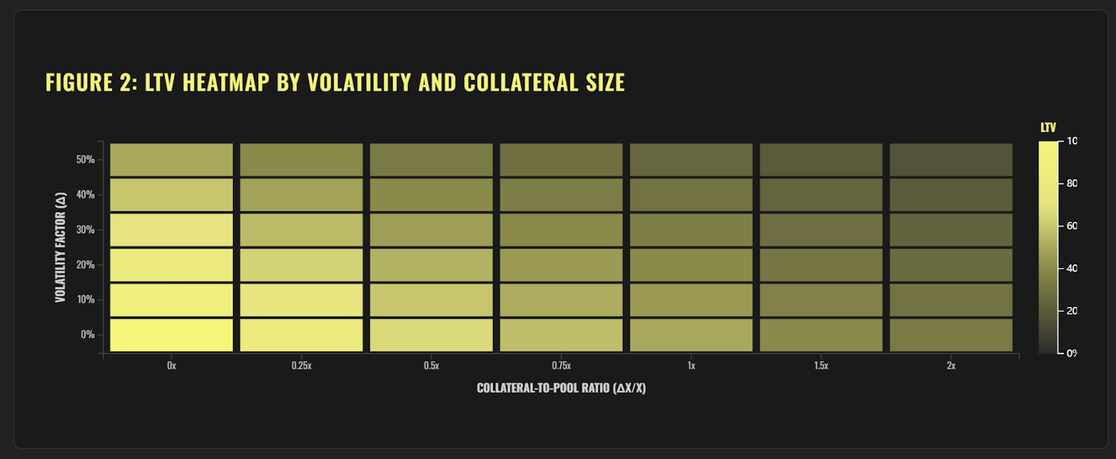
La tabla a continuación resume cómo se ajusta LTV en diferentes escenarios basados en la volatilidad y la profundidad del pool:


Fuente: Tulipán Volador
Impacto del Ajuste Dinámico de LTV en la Utilización y Liquidez
Cuando los usuarios toman prestado el activo B depositando el activo A, la composición del grupo de activos cambia. A medida que se realizan más préstamos, la liquidez disponible de B disminuye, mientras que la reserva de A aumenta, lo que hace que el grupo esté fuertemente ponderado en A.
Una alta utilización de B implica que cualquier nueva liquidación enfrentará un mayor deslizamiento (ya que Y se hace más pequeño, X crece más).
En el modelo, el estado actual del pool (X, Y) influye directamente en el LTV de los nuevos préstamos. La tasa de utilización de B (UB) se define como:
UB = 1 - (Y_actual / Y_inicial)
Cuando UB se acerca a 1, indica que la mayor parte del activo B ha sido utilizado y que la reserva está cerca de agotarse. Esto crea un grupo AMM severamente desequilibrado, donde el precio de A cae bruscamente. Si la liquidación ocurre bajo estas condiciones, el valor recuperable de B puede desplomarse.
Para contrarrestar esto, el modelo introduce un mecanismo para amortiguar el LTV en escenarios de alta utilización. Por ejemplo, si se ha utilizado el 50% de la liquidez de B, entonces solo se permite que los nuevos préstamos utilicen el 50% del límite normal de LTV.
LTVpermitido(UB) = LTVmáx × (1−UB)
Este modelo garantiza que los nuevos préstamos no agoten en exceso la liquidez disponible ni expongan los préstamos existentes a un mayor riesgo. El protocolo también puede prohibir que cualquier préstamo único consuma más de un cierto porcentaje de las reservas de B restantes. Además, el sistema puede aumentar las tarifas o las tasas de interés en condiciones de alta utilización para desalentar los préstamos más allá de los umbrales seguros, lo que forma parte de la estrategia general de gestión del riesgo de la plataforma.
A través de visualizaciones y modelización, queda claro que a medida que aumenta la volatilidad o crece el tamaño anticipado del préstamo, el rango seguro de LTV se estrecha. Esto ilustra la ventaja del modelo de LTV ajustado dinámicamente de Flying Tulip sobre los AMM tradicionales, donde las reglas estáticas a menudo no responden a las condiciones del mercado.
Fuente: Tulipán Volador
Ventajas del modelo
El modelo dinámico LTV-AMM integra deslizamiento, utilización, liquidez y volatilidad para permitir ajustes de LTV en tiempo real. Este diseño ofrece ventajas significativas en gestión de riesgos, estabilidad del sistema, eficiencia de capital y experiencia del usuario, lo que lo convierte en una solución innovadora en el espacio de préstamos DeFi.
Ajuste Dinámico
El modelo ajusta automáticamente la relación LTV basándose en las condiciones del mercado en tiempo real, asegurando que los límites de endeudamiento permanezcan alineados con la liquidez y la volatilidad.
Ejemplo: cuando la volatilidad del mercado aumenta, el LTV se reduce automáticamente para mitigar el riesgo de Gate.io.
Gestión de riesgos
Al tener en cuenta el deslizamiento y la utilización, el modelo reduce significativamente el riesgo de liquidación:
- Deslizamiento: Reduce las pérdidas por caídas de precios durante grandes liquidaciones de garantías.
- Utilización: Reduce el LTV cuando la demanda de préstamos aumenta y la utilización del pool se incrementa, evitando la sobrecarga del sistema.
Adaptación de Volatilidad
El modelo ajusta LTV en función de la volatilidad del activo:
- Activos de baja volatilidad (por ejemplo, stablecoins): LTV más alto, préstamos más fáciles.
- Activos de alta volatilidad (por ejemplo, tokens volátiles): Reduzca el LTV para gestionar el riesgo.
Estabilidad del sistema
Al combinar los factores de deslizamiento, utilización, liquidez y volatilidad, el protocolo permanece estable incluso bajo estrés del mercado, lo que ayuda a evitar el riesgo sistémico.
Eficiencia de capital
Dentro de los límites seguros, el modelo maximiza los límites de endeudamiento y mejora la utilización de capital.
Por ejemplo, cuando los mercados son estables, el LTV puede aumentarse para respaldar más préstamos.
Transparencia
La lógica del modelo es abierta y rastreable. Los usuarios pueden entender claramente cómo cambia el LTV con la dinámica del mercado, construyendo una mayor confianza en el protocolo.
Adaptabilidad
Funciona en diversas condiciones del mercado y tipos de activos, ya sea establecoins o tokens de alta volatilidad, con asignaciones razonables de LTV para cada uno.
Innovación
Al fusionar los mecanismos del creador de mercado automatizado (AMM) con la lógica de préstamos, el modelo introduce una ventaja competitiva única en DeFi, ofreciendo a los usuarios una experiencia de préstamo más segura y eficiente en capital.
Riesgos
Si bien el modelo LTV-AMM dinámico ofrece fortalezas en el control de riesgos y la resiliencia del sistema, también introduce complejidad, alta dependencia de datos, intensidad computacional y vulnerabilidad a la manipulación. Los desarrolladores deben mitigar estos riesgos a través de la optimización de parámetros, transparencia y auditorías rigurosas para garantizar la seguridad y confiabilidad.
Errores de previsión
Predicciones de volatilidad incorrectas pueden llevar a LTVs que son demasiado altos o demasiado bajos, comprometiendo la seguridad del protocolo de préstamo.
Alta dependencia de datos
El modelo depende en gran medida de datos en tiempo real (por ejemplo, precios de activos, profundidad de la piscina, tasas de utilización). Si los datos son inexactos, están retrasados o faltan, el ajuste dinámico del LTV puede fallar.
Problemas de calidad de datos
En DeFi, los datos en cadena pueden ser manipulados (por ejemplo, a través de ataques de precio), lo que podría comprometer la integridad del modelo.
Tensión en el rendimiento del sistema
Los cálculos en tiempo real del deslizamiento, la utilización y la volatilidad requieren recursos informáticos significativos, lo que potencialmente ralentiza las operaciones del sistema y degrada la experiencia del usuario.
Sensibilidad de los parámetros
La eficacia del modelo está estrechamente vinculada a la sintonización de parámetros (por ejemplo, descuentos de volatilidad, umbrales de liquidación). Los parámetros mal configurados pueden llevar a ajustes ineficaces del LTV.
Complejidad de ajuste
Encontrar combinaciones óptimas de parámetros requiere pruebas e iteraciones extensas, lo que aumenta la complejidad del desarrollo y el mantenimiento.
Congestión de red
Durante la congestión de blockchain, las actualizaciones del modelo en tiempo real pueden retrasarse, aumentando la exposición al riesgo para prestatarios y prestamistas.
Artículos relacionados

Todo lo que necesitas saber sobre Blockchain

¿Qué es Stablecoin?

¿Qué es la agricultura de liquidez?

Explicación detallada de Yala: Construyendo un Agregador de Rendimiento DeFi Modular con $YU Stablecoin como Medio

¿Qué es Neiro? Todo lo que necesitas saber sobre NEIROETH en 2025
